Consistency in Test batsmen: a new look
A statistical analysis of consistency among Test batsmen
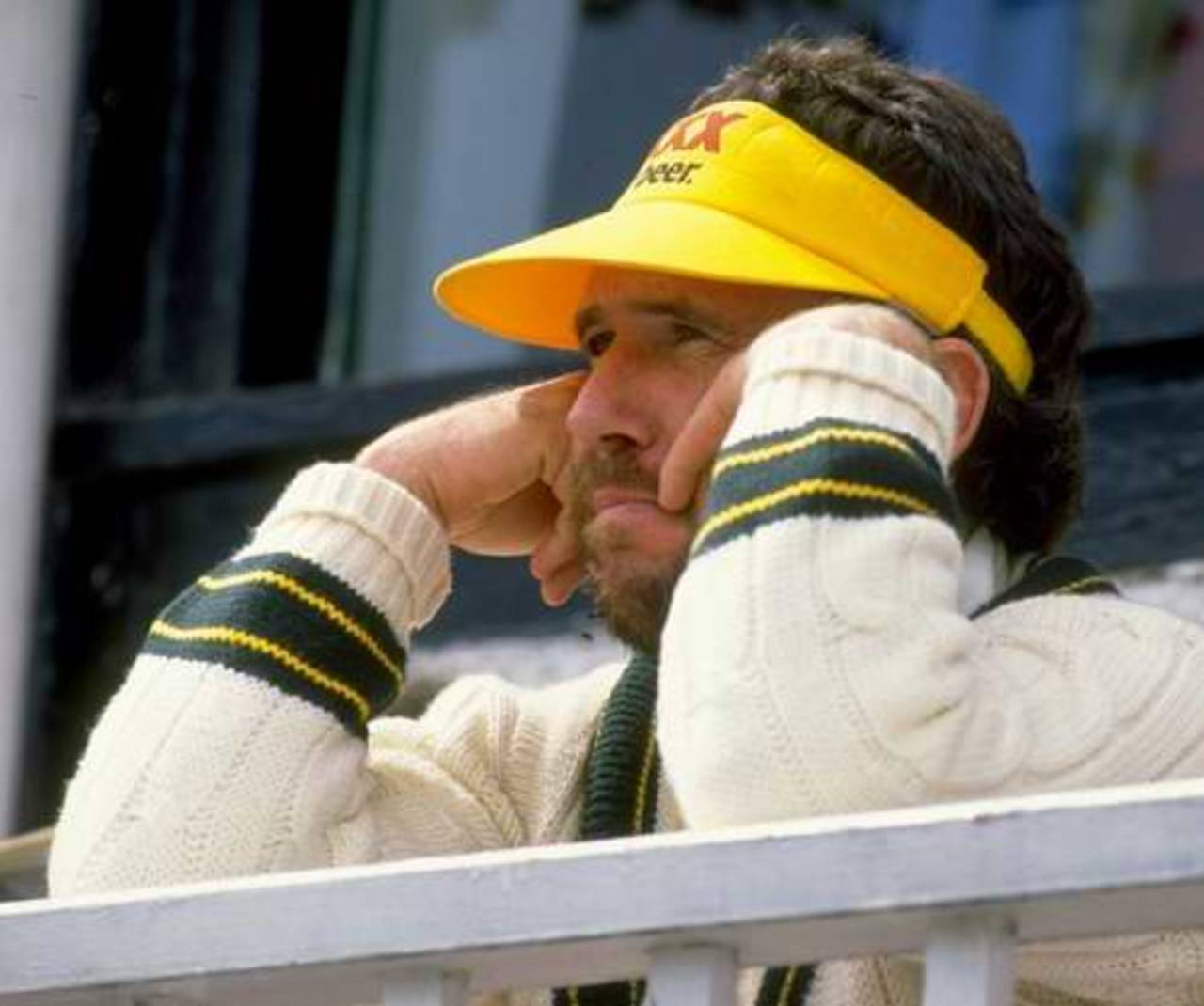
Allan Border has the lowest standard deviation among the top-20 batsmen • Adrian Murrell/Getty Images
This is based on an idea given by Prashanth. After giving the idea and participating in a discussion or two, he disappeared off the radar. However I thank him for providing the spark.
1. I had used 5 Tests as the basis for bowling. However there are many Tests in which a batsman does not get a chance to bat, because of heavy top-order batting, innings wins, big wicket wins et al. Hence I have taken 10-Innings slices as the basis for batsmen analysis. This is a reasonable number and normally covers 2-3 months of Test cricket. This is normally 5-6 Tests.
2. 10 innings means that batsman can go through a Test or two of limited opportunities to bat or non-batting because of emphatic wins etc. There will be enough opportunities within the 10-innings slice to catch up.
3. There is enough time to get over short duration loss of form.
4. To measure consistency, only runs scored will be used. The fundamental cricket dictum that batsmen should score runs and bowlers should take wickets is followed. Averages are important mainly over a career and for comparisons across players.
5. Why not average? Let us take couple of examples to understand why not. Sehwag and Younis Khan have career averages just over 50 and RpT values of around 85. In a 10-innings period, match context being comparable, Younis scores 330 at 55 and Sehwag scores 450 at 45. Who has performed closer to his career figures and for that matter, better. Certainly Sehwag, despite the lower slice average.
6. Let us not forget that we remember numbers like 974 (Bradman), 774 (Gavaskar) and 688 (Lara) rather than the averages.
7. The career slices should be non-overlapping and equal, other than the last one. Gooch's 333 should be part of one career slice only. Hence the concept of rolling number of innings is not valid.
8. 10 innings might seem arbitrary but represents a long enough career slice. It represents a long 5/6 Test series.
9. The keyword is consistency with reference to the player's own career performance levels.
10. We are not looking about high and low values but only relative to the concerned player's career figures. Over a 10-innings stretch Graeme Smith is expected to score 408 runs and Habibul Bashar is expected to score 300 runs. This will be the basis. If Smith scored 350 runs, it is a below-average performance and if Bashar scored 350 runs, it is an above-average performance.
11. Adjustment is made for the last career slice if the same is fewer than 10 innings.
12. The criteria for selection is 3000 or more Test runs. 162 batsmen qualify. It is unfortunate that a few top batsmen like Graeme Pollock and George Headley do not make the cut.
14.The Standard Deviation (SD) of the slice ratios is used to determine consistency.
15.There were suggestions that I should use more Tests/innings as the basis. I have resisted that idea mainly because I want to be hard on the players. If English batsmen had a great five- Test stint in summer and a poor five-Test sojourn in winter, I want these to be treated as two out-of-the-normal occurrences and do not want to get the 10 Tests together, get a nice, middle-level performance which papers over cracks. Same with all teams. Let us also agree. If a batsman scores 180 runs in 10 innings, it is a major cause for concern and should not be covered up by 600 runs in 10 innings before or after this barren period..
The following 5 groups are formed for purposes of determining consistency. For each career-slice of 10-innings, a ratio is formed between that concerned slice's runs and the career-average runs for 10 tests. This ratio is called SPF (Slice Performance Factor). Suppose the batsman has scored 284 runs and his 10-innings and his career-RpI value is 40, the SPF value is 0.71. If he scored 501 runs, the SPF is 1.25.
A. SPF  below 0.67:  Well below average - Falls into the inconsistent bracket.
B. SPF 0.67 - 0.90:  Below average
C. SPF 0.90 - 1.10:  Around average
D. SPF 1.10 - 1.33:  Above average
E. SPF  above 1.33:  Well above average - Falls into the inconsistent bracket.
First some data tables. The complete table is available for download. The tables and graphs are presented with least comments. Let me allow the erudite readers to come out with their own comments.
| Batsman | Team | Innings | Runs | Avge | RpI | Mean | StdDev | Mid3% | Grps | Grp A | Grp B | Grp C | Grp D | Grp E |
|---|---|---|---|---|---|---|---|---|---|---|---|---|---|---|
| % | <67 | 67-90 | 90-110 | 110-133 | >133 | |||||||||
| Tendulkar S.R | Ind | 311 | 15470 | 55.45 | 49.7 | 0.99 | 0.325 | 68.8 | 32 | 4 | 10 | 7 | 5 | 6 |
| Dravid R | Ind | 286 | 13288 | 52.31 | 46.5 | 0.99 | 0.332 | 72.4 | 29 | 4 | 9 | 5 | 7 | 4 |
| Ponting R.T | Aus | 276 | 13196 | 53.43 | 47.8 | 1.01 | 0.412 | 60.7 | 28 | 5 | 5 | 8 | 4 | 6 |
| Kallis J.H | Saf | 257 | 12379 | 56.78 | 48.2 | 1.00 | 0.348 | 69.2 | 26 | 4 | 5 | 6 | 7 | 4 |
| Lara B.C | Win | 232 | 11953 | 52.89 | 51.5 | 0.99 | 0.278 | 75.0 | 24 | 3 | 8 | 3 | 7 | 3 |
| Border A.R | Aus | 265 | 11174 | 50.56 | 42.2 | 0.99 | 0.241 | 81.5 | 27 | 2 | 6 | 10 | 6 | 3 |
| Waugh S.R | Aus | 260 | 10927 | 51.06 | 42.0 | 1.00 | 0.333 | 61.5 | 26 | 4 | 7 | 5 | 4 | 6 |
| Jayawardene D.P | Slk | 217 | 10443 | 51.19 | 48.1 | 1.00 | 0.352 | 59.1 | 22 | 5 | 4 | 4 | 5 | 4 |
| Gavaskar S.M | Ind | 214 | 10122 | 51.12 | 47.3 | 1.00 | 0.350 | 68.2 | 22 | 4 | 6 | 4 | 5 | 3 |
| Chanderpaul S | Win | 234 | 9709 | 49.28 | 41.5 | 1.01 | 0.304 | 66.7 | 24 | 4 | 5 | 5 | 6 | 4 |
| Sangakkara K.C | Slk | 183 | 9382 | 54.87 | 51.3 | 0.99 | 0.425 | 57.9 | 19 | 4 | 4 | 5 | 2 | 4 |
| Gooch G.A | Eng | 215 | 8900 | 42.58 | 41.4 | 0.99 | 0.363 | 72.7 | 22 | 4 | 5 | 6 | 5 | 2 |
| Javed Miandad | Pak | 189 | 8832 | 52.57 | 46.7 | 1.00 | 0.384 | 57.9 | 19 | 3 | 6 | 4 | 1 | 5 |
| Inzamam-ul-Haq | Pak | 200 | 8830 | 49.61 | 44.1 | 1.00 | 0.376 | 60.0 | 20 | 5 | 3 | 3 | 6 | 3 |
| Laxman V.V.S | Ind | 225 | 8781 | 45.97 | 39.0 | 0.99 | 0.307 | 69.6 | 23 | 3 | 7 | 6 | 3 | 4 |
| Hayden M.L | Aus | 184 | 8626 | 50.74 | 46.9 | 0.99 | 0.385 | 47.4 | 19 | 6 | 1 | 6 | 2 | 4 |
| Richards I.V.A | Win | 182 | 8540 | 50.24 | 46.9 | 0.99 | 0.406 | 73.7 | 19 | 2 | 7 | 6 | 1 | 3 |
| Stewart A.J | Eng | 235 | 8465 | 39.56 | 36.0 | 1.00 | 0.368 | 66.7 | 24 | 4 | 6 | 6 | 4 | 4 |
| Gower D.I | Eng | 204 | 8231 | 44.25 | 40.3 | 0.99 | 0.297 | 85.7 | 21 | 2 | 7 | 6 | 5 | 1 |
| Sehwag V | Ind | 167 | 8178 | 50.80 | 49.0 | 0.99 | 0.428 | 52.9 | 17 | 4 | 5 | 3 | 1 | 4 |
| Boycott G | Eng | 193 | 8114 | 47.73 | 42.0 | 0.99 | 0.332 | 70.0 | 20 | 3 | 4 | 6 | 4 | 3 |
| Smith G.C | Saf | 174 | 8043 | 49.65 | 46.2 | 0.99 | 0.350 | 66.7 | 18 | 2 | 8 | 2 | 2 | 4 |
| Sobers G.St.A | Win | 160 | 8032 | 57.78 | 50.2 | 1.00 | 0.307 | 68.8 | 16 | 3 | 3 | 4 | 4 | 2 |
| Waugh M.E | Aus | 209 | 8029 | 41.82 | 38.4 | 1.00 | 0.283 | 76.2 | 21 | 2 | 6 | 6 | 4 | 3 |
| Fleming S.P | Nzl | 189 | 7172 | 40.07 | 37.9 | 1.00 | 0.247 | 84.2 | 19 | 1 | 8 | 4 | 4 | 2 |
| Chappell G.S | Aus | 151 | 7110 | 53.86 | 47.1 | 1.00 | 0.255 | 81.2 | 16 | 2 | 4 | 2 | 7 | 1 |
| Bradman D.G | Aus | 80 | 6996 | 99.94 | 87.5 | 1.00 | 0.272 | 75.0 | 8 | 1 | 2 | 1 | 3 | 1 |
| Flower A | Zim | 112 | 4794 | 51.55 | 42.8 | 0.98 | 0.436 | 66.7 | 12 | 2 | 4 | 4 | 0 | 2 |
To clarify the table contents. RpI mean Runs per innings. Mean is the mean of the SPF values and is close to 1.0 for all batsmen. StdDev is the Standard Deviation for all the SPF values. Mid3% is the % of the Groups B, C and D over the total number of Career Slices, which is the next column: Grps. Grp A to Grp E are self-explanatory. The complete file is available for downloading. The link is provided at the end. The first one is the core table of batsmen who have scored over 8000 runs in their Test career. In addition, Don Bradman (no need to explain), Greg Chappell (a modern great), Stephen Fleming (New Zealand) and Andy Flower (Zimbabwe) are included.
Contrary to what all of us may have perceived, Lara is remarkably consistent on this 10-innings basis. His SD of 0.278 is second only to Border amongst the top-20 batsmen. Just to confirm that this is not a fluke, look at his Mid3% which is quite high at 75.2. Again, bettered only by Border and Gower.
Consistency is determined in two ways. The first is statistical. The Standard Deviation (SD) is determined for all the ratios. Low SD values indicate consistent players and high SD values indicate inconsistent players. The usual method of using the Coefficient of Variation is not required since the means for almost all players is around 1.00. Shown below are the SD tables with the low-20 SDs indicating very consistent batsmen.
| Batsman | Team | Innings | Runs | Avge | RpI | Mean | StdDev | Mid3% | Grps | Grp A | Grp B | Grp C | Grp D | Grp E |
|---|---|---|---|---|---|---|---|---|---|---|---|---|---|---|
| % | <67 | 67-90 | 90-110 | 110-133 | >133 | |||||||||
| Greig A.W | Eng | 93 | 3599 | 40.44 | 38.7 | 0.99 | 0.171 | 100.0 | 10 | 0 | 2 | 5 | 3 | 0 |
| Redpath I.R | Aus | 120 | 4737 | 43.46 | 39.5 | 1.00 | 0.195 | 91.7 | 12 | 0 | 4 | 4 | 3 | 1 |
| Ranatunga A | Slk | 155 | 5105 | 35.70 | 32.9 | 1.01 | 0.202 | 93.8 | 16 | 0 | 7 | 4 | 4 | 1 |
| Hassett A.L | Aus | 69 | 3073 | 46.56 | 44.5 | 0.99 | 0.204 | 85.7 | 7 | 1 | 1 | 2 | 3 | 0 |
| Fredericks R.C | Win | 109 | 4334 | 42.49 | 39.8 | 1.00 | 0.205 | 100.0 | 11 | 0 | 3 | 4 | 4 | 0 |
| Pietersen K.P | Eng | 143 | 6654 | 49.29 | 46.5 | 1.01 | 0.210 | 86.7 | 15 | 1 | 3 | 7 | 3 | 1 |
| Knott A.P.E | Eng | 149 | 4389 | 32.75 | 29.5 | 1.00 | 0.228 | 86.7 | 15 | 1 | 4 | 5 | 4 | 1 |
| Saeed Anwar | Pak | 91 | 4052 | 45.53 | 44.5 | 1.02 | 0.230 | 100.0 | 10 | 0 | 4 | 1 | 5 | 0 |
| Smith R.A | Eng | 112 | 4236 | 43.67 | 37.8 | 1.00 | 0.236 | 83.3 | 12 | 1 | 4 | 4 | 2 | 1 |
| Hutton L | Eng | 138 | 6971 | 56.67 | 50.5 | 0.99 | 0.237 | 85.7 | 14 | 1 | 5 | 2 | 5 | 1 |
| Wright J.G | Nzl | 148 | 5334 | 37.83 | 36.0 | 1.00 | 0.238 | 80.0 | 15 | 1 | 6 | 2 | 4 | 2 |
| Border A.R | Aus | 265 | 11174 | 50.56 | 42.2 | 0.99 | 0.241 | 81.5 | 27 | 2 | 6 | 10 | 6 | 3 |
| Ijaz Ahmed | Pak | 92 | 3315 | 37.67 | 36.0 | 0.98 | 0.246 | 90.0 | 10 | 0 | 4 | 2 | 3 | 1 |
| Fleming S.P | Nzl | 189 | 7172 | 40.07 | 37.9 | 1.00 | 0.247 | 84.2 | 19 | 1 | 8 | 4 | 4 | 2 |
| Mushtaq Mohammad | Pak | 100 | 3643 | 39.17 | 36.4 | 1.00 | 0.248 | 70.0 | 10 | 1 | 3 | 2 | 2 | 2 |
| Hunte C.C | Win | 78 | 3245 | 45.07 | 41.6 | 1.00 | 0.248 | 87.5 | 8 | 0 | 3 | 3 | 1 | 1 |
| Collingwood P.D | Eng | 115 | 4260 | 40.57 | 37.0 | 0.98 | 0.249 | 91.7 | 12 | 1 | 3 | 4 | 4 | 0 |
| Strauss A.J | Eng | 167 | 6604 | 41.02 | 39.5 | 1.00 | 0.250 | 82.4 | 17 | 0 | 9 | 2 | 3 | 3 |
| Sutcliffe H | Eng | 84 | 4555 | 60.73 | 54.2 | 0.98 | 0.252 | 77.8 | 9 | 1 | 2 | 4 | 1 | 1 |
| Chappell G.S | Aus | 151 | 7110 | 53.86 | 47.1 | 1.00 | 0.255 | 81.2 | 16 | 2 | 4 | 2 | 7 | 1 |
Tony Greig is the surprise leader in this table, with a low SD value of 0.171. The most notable modern batsman in this table is Pietersen with an excellent SD value 0.210. Other than Pietersen there is no current batsman in this list. Like Lara. he has certainly surprised us. Maybe there is a lot of substance behind that exaggerated swagger. He talked about the many hours of practice put in while talking of his Colombo classic. Maybe that is paying off. It is also possible that unlike what one associates with him, he does not have extensive bad patches nor purple patches. I also wish he stops making silly statements.
The alternate method is common-sense-based rather than on a statistical measure. The two extreme group numbers, A and E, are considered significant departures from the career levels. The middle three group numbers are added and divided by the total number of slices to get the Mid3%. This reflects the consistency of the players. Shown below are the SD tables with the high-10 Mid3% values.
| Batsman | Team | Innings | Runs | Avge | RpI | Mean | StdDev | Mid3% | Grps | Grp A | Grp B | Grp C | Grp D | Grp E |
|---|---|---|---|---|---|---|---|---|---|---|---|---|---|---|
| % | <67 | 67-90 | 90-110 | 110-133 | >133 | |||||||||
| Fredericks R.C | Win | 109 | 4334 | 42.49 | 39.8 | 1.00 | 0.205 | 100.0 | 11 | 0 | 3 | 4 | 4 | 0 |
| Saeed Anwar | Pak | 91 | 4052 | 45.53 | 44.5 | 1.02 | 0.230 | 100.0 | 10 | 0 | 4 | 1 | 5 | 0 |
| Greig A.W | Eng | 93 | 3599 | 40.44 | 38.7 | 0.99 | 0.171 | 100.0 | 10 | 0 | 2 | 5 | 3 | 0 |
| Ranatunga A | Slk | 155 | 5105 | 35.70 | 32.9 | 1.01 | 0.202 | 93.8 | 16 | 0 | 7 | 4 | 4 | 1 |
| Redpath I.R | Aus | 120 | 4737 | 43.46 | 39.5 | 1.00 | 0.195 | 91.7 | 12 | 0 | 4 | 4 | 3 | 1 |
| Collingwood P.D | Eng | 115 | 4260 | 40.57 | 37.0 | 0.98 | 0.249 | 91.7 | 12 | 1 | 3 | 4 | 4 | 0 |
| Ijaz Ahmed | Pak | 92 | 3315 | 37.67 | 36.0 | 0.98 | 0.246 | 90.0 | 10 | 0 | 4 | 2 | 3 | 1 |
| Hunte C.C | Win | 78 | 3245 | 45.07 | 41.6 | 1.00 | 0.248 | 87.5 | 8 | 0 | 3 | 3 | 1 | 1 |
| Pietersen K.P | Eng | 143 | 6654 | 49.29 | 46.5 | 1.01 | 0.210 | 86.7 | 15 | 1 | 3 | 7 | 3 | 1 |
| Knott A.P.E | Eng | 149 | 4389 | 32.75 | 29.5 | 1.00 | 0.228 | 86.7 | 15 | 1 | 4 | 5 | 4 | 1 |
| Gower D.I | Eng | 204 | 8231 | 44.25 | 40.3 | 0.99 | 0.297 | 85.7 | 21 | 2 | 7 | 6 | 5 | 1 |
| Cook A.N | Eng | 135 | 6184 | 48.69 | 45.8 | 1.00 | 0.291 | 85.7 | 14 | 1 | 5 | 5 | 2 | 1 |
| Hutton L | Eng | 138 | 6971 | 56.67 | 50.5 | 0.99 | 0.237 | 85.7 | 14 | 1 | 5 | 2 | 5 | 1 |
| Slater M.J | Aus | 131 | 5312 | 42.84 | 40.5 | 0.98 | 0.263 | 85.7 | 14 | 1 | 4 | 4 | 4 | 1 |
| Hassett A.L | Aus | 69 | 3073 | 46.56 | 44.5 | 0.99 | 0.204 | 85.7 | 7 | 1 | 1 | 2 | 3 | 0 |
These are the batsmen with high middle three group % values indicating a high degree of consistency. In the bowler tables, there were six bowlers with 100% of their groups in the middle-3 groups. It seems like batting is slightly more difficult since there are only three batsmen. These all belong to the 70s/80s/90s. Roy Fredericks, the attacking West Indian batsman leads the three-some, followed by Saeed Anwar and Tony Greig. Collingwood is there as also Pietersen and Cook. Possible reason for England's pre-eminence.
Now for some special graphs.
Top run-scoring batsmen
 Top run-getters in Tests career
© Anantha Narayanan
The top-9 batsmen, who have crossed 10000 Test runs, are featured. It can be clearly seen that most of these batsmen do not exhibit a high level of consistency. The only exceptions seem to be Allan Border and for the first two-thirds of his career, Jayawardene.
Most consistent: Based on low SD values
 batsmen with low standard deviation values
© Anantha Narayanan
As already discussed this table is led by Tony Greig. A fairly low SD of 0.171 indicates a very consistent career. This is borne out by his placement in the next graph also. However it should be noted that the lowest SD value for bowlers is a much lower 0.124. Pietersen finds a place in both the consistency graphs.
Most consistent: Based on high Middle-3-group % values
 Batsmen with high middle-3 group % values
© Anantha Narayanan
Unlike bowlers where there were six with 100% in the middle categories, amongst batsmen, there are only three: namely Fredericks, Saeed Anwar and Greig.
Least consistent: Based on high SD values
These graphs look like the dying person's cardiograph. These batsmen have had moves up and down throughout their career. Exemplified by Gambhir who had a poor start, great move up and then fell off equally badly. Vettori has had such a Jekyll and Hide career that it is not surprising to see him here. In the first 70 innings Vettori averaged 18. In the next 100 innings he averaged well over 35.
Least consistent: Based on low Middle-3-group % values
 Batsmen with low middle-3 % values
© Anantha Narayanan
It is clear that these two methods of determining consistency are quite different. There are different sets of batsmen in the two graphs.
Batsmen with top RpI figures
 Batsmen with highest RPI figures
© Anantha Narayanan
Just to complete the analysis I have given here the charts for the top batsmen - by Runs per innings, since most of them would have missed the first chart: by career runs scored. Again inconsistency seems to be the trend here.
I think mention must be made of two batsmen, Tony Greig and Kevin Pietersen. Tony Greig never went off the middle three groups. That is some level of consistency. Pietersen, amongst the modern batsmen, has surprised us with his high degree of consistency.
To download/view the Excel sheet containing the complete data for 162 batsmen please click/right-click here. I have strengthened the Excel sheet by colour coding the individual SPF values through dynamic formatting.
Ed Smith's thought-provoking piece on randomness and form "When is poor form just randomness?" (click here) made me realize that this particular measure I have created can be applied to Ed Smith's axiom. Suppose I summed the SPF values of the top six batsmen or top four bowlers for every Test/innings, we would know what are the lowest SPF averages (very poor form, as a group of six/four players) and the highest SPF averages (very rich form, as a group of six/four players). That, for a later article.
Anantha Narayanan has written for ESPNcricinfo and CastrolCricket and worked with a number of companies on their cricket performance ratings-related systems