What median scores tell us about batting careers
While the average is the more common stat by which batting numbers are measured, looking at metrics based on the median throws up some interesting findings
Anantha Narayanan
14-Apr-2018
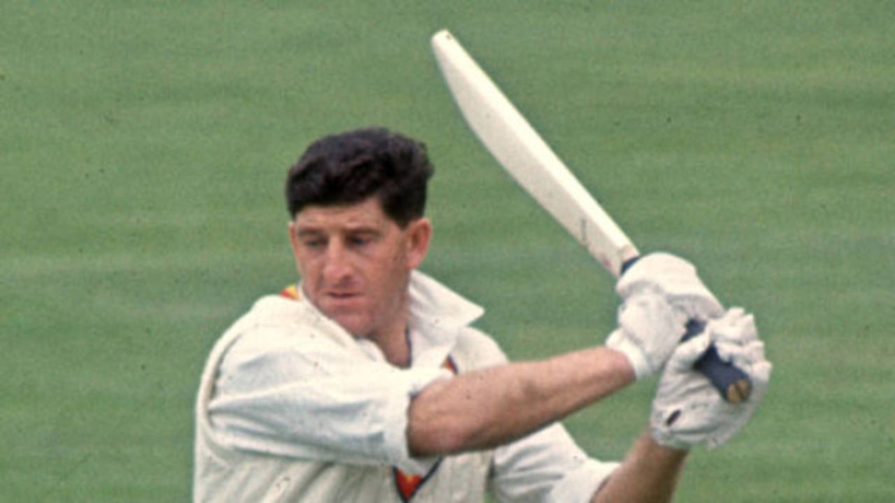
Kevin Barrington's median is an impressive 46 - striking for someone whose batting average was 58 • Getty Images
Some caveats to start with. I am a cricket analyst, not a statistician. I have not studied statistics. I have not worked in statistics-related positions. My knowledge of statistics is from what I learnt taking a course at IBM, and subsequently through general interest. Having got that off my chest, I can safely go on to this article with the firm knowledge that my common-sense-based application of statistical measures here will not invite comments relating to my qualifications.
The spark for this article came from a reference to the median by S Rajesh in his stats review at the end of the Ashes series. He compared the series performance of the two leading English batsmen. Joe Root scored 378 runs at 47.25, and Alastair Cook an almost identical tally of 376 runs at 47.00. But the two efforts were chalk and cheese. The median score for Root was 51 (1, 9, 14, 15, 51, 58, 61, 67, 83) and that for Cook was 14 (2, 7, 7, 10, 14, 16, 37, 39, 244). This showed how lopsided Cook's performance was. It made me wonder how the top batsmen in the game had fared on this measure through their careers. This article is the result.
Incidentally, my friend Kartikeya Date covered the idea of the median in a blog post. However, he did this four years ago, when Steve Smith's career was just about stabilising at 1361 runs at an average of 40. So a lot of water has passed under London Bridge, and in any case, my look at the median is different to Kartikeya's. But let me acknowledge his pioneering effort, and that of anyone else who has done this sort of analysis before.
Before continuing, let me assure readers that this is not a heavy, theory-based article. Whatever terms I use, I will immediately demonstrate with simple diagrams.
What is a median? Very simple. It is the score that stands exactly in the middle of an ordered list of values. If there are an odd number of performances, the median is the exact middle value. If there are an even number of performances, it is the average of the two values in the middle.
As usual, first let me define the selection criteria. I have set 3000 Test runs as the minimum qualifying mark. To score 3000 Test runs, batsmen have to play between 30 and 50 Tests, and that defines a sufficiently long career. What about batting average? A single batsman, Shane Warne, has scored in excess of 3000 Test runs at a batting average below 20. I decided to keep the blond bowling genius in. As such, 189 batsmen qualify.
That was just the raw data. Now to derive some insights. By now, we all know that the median is in the exact middle. The key question is: where is the mean? And by the by, what is the mean? It is certainly not the batting average, which is a derived measure for cricket, since it involves not-outs. Only here can an innings of six hours suddenly cease to exist. The batting average is certainly a lovely measure but it is not the mean.
The mean is developed by dividing the number of runs by the number of innings. By the way, the RpAI, which is one of my favourite measures, is, like the batting average, a derived measure. The mean is the raw RpAI. And it is clear that, for all batsmen, without exception, across their careers the mean will be greater than the median. This is simple logic. All batting distributions will have more scores below the mean than above. If the mean is 50, the presence of a score of 200 would mean that of three scores of zeroes. A score of 300 would imply five zeroes.
Median-Mean Ratio (MMR): Let us look at the ratio of median to mean. This is not a standard statistical measure. I would term it a common-sense measure to get an idea of how separated the mean and median are. Let me fix the mean at 50.
In the first case we are looking at, let the median and mean be exactly the same. This is the perfect distribution. There are as many scores below the mean as there are above it. It could happen in a series but never across a career. The MMR is around 1.0. Suppose the median is 10 (similar to Cook in the Ashes series). This indicates that there were many small scores below the median but all these were compensated by one (or possibly two) high scores. Say, 0, 0, 0, 10, 20, 110 and 210. The MMR would be 0.2, indicating that the median is some distance from the mean.
Let us say the median is 40, possibly from a range of scores like 0, 10, 20, 40, 70, 100 and 110. This can only happen with a mix of close numbers on either side of the median. The MMR is 0.80. It is possible for this to happen across long careers and indicates a very consistent career.
Let us say the median is 80. How can this happen? Possibly scores like 0, 0, 0, 80, 85, 90 and 95. Notice that Root's numbers from the Ashes are similar. This can only happen with a mix of very low numbers on the one side and numbers very close to the median on the other. The MMR is 1.60 here. Impossible for this to happen across long careers.
Now imagine two distributions. The first one is 0, 10, 20, 40, 70, 100 and 110. The second one is 25, 30, 35, 40, 65, 70 and 85. The mean (50) and median (40) values of both distributions are the same. The MMR for both distributions is 0.80. However, the two distributions are quite different. The first is a more widely spread distribution, while the second is a closely bunched distribution. This difference is quantified by the standard deviation (SD). The SD for the first distribution is 44.0 and the for the second one, 23.1. Therefore I would want an alternative measure involving the mean, median and standard deviation.
Pearson's Skew Coefficient-2 (PSC-2)
That measure is the Pearson's Skew Coefficient-2, which is median-based. The formula to derive the PSC-2 is:
That measure is the Pearson's Skew Coefficient-2, which is median-based. The formula to derive the PSC-2 is:
3 * (Mean - Median) / Standard Deviation
The PSC-2 values for the two distributions described above are 0.682 and 1.298 respectively. These two numbers are quite different.
How would one interpret PSC-2? The PSC-2 value indicates the skew of the distribution. A PSC-2 value of 0.0 indicates a perfectly balanced normal distribution in which the mean, median (and the mode) are equal. A positive PSC-2 value (mean greater than the median) indicates a positively skewed distribution in which there is a concentration of values on the left, below the median value. This is the distribution for all batsmen through their careers. The magnitude of PSC-2 indicates the degree of positive skew. High values indicate more unbalanced distributions. A negative PSC-2 value (mean lower than the median) indicates a negatively skewed distribution in which there is a concentration of values on the right, above the median value.
From the above two images, it is clear that all distributions of batsmen's scores across a career will be positively skewed, that is, more of them will be on the left. There will be no exceptions, barring the likes of, say, a three-innings career where the scores are 10, 50, 60. Batsmen are likely to have a lot more scores in class intervals like 0-4 and 5-9 than in, say, 100-104 or 200-204. However, within a shorter span like a series, there is a possibility of a negatively skewed distribution. It is interesting to note that Root's performance in the Ashes series was negatively skewed (median greater than mean).
At this stage, let us look at some overall numbers for the population of 189 batsmen who have scored 3000-plus Test runs.
Mean: Average - 39.45. Mid value - 39.6.
Median: Average - 25.6. Mid value - 26.0.
PSC-2: Average - 0.982. Mid value - 0.980.
MMR: Average - 0.648. Mid value - 0.650.
Median: Average - 25.6. Mid value - 26.0.
PSC-2: Average - 0.982. Mid value - 0.980.
MMR: Average - 0.648. Mid value - 0.650.
When seen across the entire population, note how close the average (mean) and the mid-value (median) values are. And refer back to these values when looking at the individual batsmen's numbers.
Let us first look at the top ten batsmen based on the median values.
| Batsman | Cty | Ins | Runs | Mean | Median |
|---|---|---|---|---|---|
| Bradman | Aus | 80 | 6996 | 87.45 | 56.5 |
| Barrington | Eng | 131 | 6806 | 51.95 | 46.0 |
| Hobbs | Eng | 102 | 5410 | 53.04 | 40.0 |
| Sutcliffe | Eng | 84 | 4555 | 54.23 | 38.0 |
| Weekes | Win | 81 | 4455 | 55.00 | 36.0 |
| Walcott | Win | 74 | 3798 | 51.32 | 34.5 |
| Smith | Aus | 117 | 6199 | 52.98 | 34.0 |
| Hassett | Aus | 69 | 3073 | 44.54 | 34.0 |
| Katich | Aus | 99 | 4188 | 42.30 | 34.0 |
| Lara | Win | 232 | 11953 | 51.52 | 33.5 |
This is a table just to get us going. Not surprisingly, Don Bradman is at the top, with a median value of 56. Just a reminder: Bradman has as many scores below 56 as he has above it. That is some career. However, it also reveals that his median value is not that high. Take the next batsman: Ken Barrington. His median is 46.0. That is an impressive value for someone whose average is 58.67 to Bradman's 99.94.
In fact, the table is occupied by batsmen with high averages/means. The top seven have averages above 56.5 and mean values above 50. Then come two surprise batsmen: Lindsay Hassett and Simon Katich. Their average is below 50 and mean below 45, but they have high median values, which indicates a more balanced career. Brian Lara rounds off the table with a median of 33.5. His mean is very close to his average because of very few not-outs.
Now a look at the bottom ten values.
| Batsman | Cty | Ins | Runs | Mean | Median |
|---|---|---|---|---|---|
| Amiss | Eng | 88 | 3612 | 41.05 | 16.0 |
| John Reid | Nzl | 108 | 3428 | 31.74 | 16.0 |
| Geoff Marsh | Aus | 150 | 3633 | 24.22 | 15.5 |
| Ijaz Ahmed | Pak | 92 | 3315 | 36.03 | 15.0 |
| Grant Flower* | Zim | 123 | 3457 | 28.11 | 15.0 |
| Vettori | Nzl | 174 | 4531 | 26.04 | 15.0 |
| Hadlee | Nzl | 134 | 3124 | 23.31 | 15.0 |
| Healy | Aus | 182 | 4356 | 23.93 | 14.0 |
| C Vaas | Slk | 111 | 3089 | 18.95 | 12.0 |
| Warne | Aus | 145 | 3154 | 15.85 | 10.0 |
It is no surprise that Warne is bottom of the table, with a very low median score of 10.0, nor that Chaminda Vaas is next to him, with a median of 12.0. Then come a few players for whom batting was a secondary function. Dennis Amiss is a surprise entry, with a low median score. The common thread between these batsmen is that they are quite inconsistent. There are many low scores and compensatory high scores.
Now let us look at the top ten batsmen based on PSC-2 values. To recap, the PSC-2 is calculated by the formula PSC-2 = 3 * (Mean-Median)/SD. As such, a low PSC-2 value will mean that the mean and median are in close proximity, and indicates a more balanced distribution, ergo a high level of consistency. A high PSC-2 value will indicate a significant distance between the mean and median, indicating the presence of a lot more low values among the scores.
| Batsman | Cty | Ins | Runs | Mean | Median | Std Devn | MMR | PSC-2 |
|---|---|---|---|---|---|---|---|---|
| Barrington | Eng | 131 | 6806 | 51.95 | 46.0 | 47.3 | .885 | 0.377 |
| Ranatunga | Slk | 155 | 5105 | 32.94 | 27.0 | 29.4 | .820 | 0.605 |
| Katich | Aus | 99 | 4188 | 42.30 | 34.0 | 37.8 | .804 | 0.660 |
| Edrich | Eng | 127 | 5138 | 40.46 | 30.0 | 45.0 | .742 | 0.697 |
| Hunte | Win | 78 | 3245 | 41.60 | 31.0 | 45.1 | .745 | 0.706 |
| Hassett | Aus | 69 | 3073 | 44.54 | 34.0 | 44.5 | .763 | 0.710 |
| Imran Khan | Pak | 126 | 3807 | 30.21 | 23.0 | 30.4 | .761 | 0.712 |
| Redpath | Aus | 120 | 4737 | 39.47 | 31.0 | 34.9 | .785 | 0.729 |
| Walters | Aus | 125 | 5357 | 42.86 | 32.0 | 44.5 | .747 | 0.731 |
| Amarnath | Ind | 113 | 4378 | 38.74 | 30.0 | 35.8 | .774 | 0.732 |
Barrington's PSC-2 value of 0.377 is so far off the next value that, in this measure, he is Bradmanesque. A high median means that these two values are close (56 v 52). The MMR, which is given here for information, is a very high 0.885. This table is full of surprises. Arjuna Ranatunga is unexpected in position two, with a PSC-2 value of 0.605. Katich and John Edrich are next in line, with PSC-2 values below 0.7. Then come a set of six batsmen, led by Imran Khan, whose PSC-2 values are between 0.7 and 0.732. A perusal of the frequency distribution graphs will make it clearer.
In order to get some clarity on the PSC-2 with respect to the batsmen's score distribution, I will show the frequency distribution graphs of some selected players. A plotting of individual scores will be meaningless, since there are too many: at last count, 329. Hence a classification is done. I tried different values before zeroing in on classes whose width is five runs each. That means I have classes 0-4, 5-9, 10-14... onwards to the last class, which varies from player to player. For Lara, it is 400-404; for Bradman, it is 330-334, for Mohammad Azharuddin, it is 195-199, and so on. The graphs are centred horizontally based on the number of classes.
First are three graphs of batsmen selected from the top ten of the PSC-2 table.
Let us first look at Barrington's graph. Look at how close the median and mean classes are. In fact, they are located next to each other. It can also be seen that the graph is not populated at all between the classes of 170-174 and the highest, 255-259.
Edrich's graph is somewhat similar to Barrington's. The interesting feature of the graph is that the most frequent class is not the first one (0-4) but the second (5-9). The median and mean classes are separated by two classes.
Doug Walters was prone to failures in the 0-4 range. However, he more than compensates with the bunching of the second class onwards. His median and mean classes are also two classes apart.
Now, the table of bottom ten values, based on PSC-2.
| Batsman | Cty | Ins | Runs | Mean | Median | Std Devn | MMR | PSC-2 |
|---|---|---|---|---|---|---|---|---|
| Cook | Eng | 279 | 12028 | 43.11 | 24.0 | 48.9 | 0.557 | 1.174 |
| ..... | ||||||||
| Pujara | Ind | 96 | 4496 | 46.83 | 27.0 | 49.4 | 0.577 | 1.205 |
| Samaraweera | Slk | 81 | 5462 | 41.38 | 23.5 | 44.2 | 0.568 | 1.213 |
| Zaheer Abbas | Pak | 124 | 5062 | 40.82 | 19.0 | 54.0 | 0.465 | 1.213 |
| N Hussain | Eng | 171 | 5764 | 33.71 | 19.0 | 36.3 | 0.564 | 1.216 |
| Lamb | Eng | 139 | 4656 | 33.50 | 19.0 | 35.7 | 0.567 | 1.219 |
| Elgar | Saf | 82 | 3194 | 38.95 | 20.5 | 43.0 | 0.526 | 1.287 |
| Asad Shafiq | Pak | 97 | 3614 | 37.26 | 21.0 | 37.7 | 0.564 | 1.293 |
| Hill | Aus | 89 | 3412 | 38.34 | 19.0 | 44.1 | 0.496 | 1.317 |
| Amiss | Eng | 88 | 3612 | 41.05 | 16.0 | 55.7 | 0.390 | 1.348 |
| Reid | Nzl | 108 | 3428 | 31.74 | 16.0 | 34.4 | 0.504 | 1.373 |
| Ijaz Ahmed | Pak | 92 | 3315 | 36.03 | 15.0 | 45.1 | 0.416 | 1.400 |
Ijaz Ahmed has the highest PSC-2 value of 1.4. The bottom 14 is a motley collection of batsmen across the ages. There are allrounders and specialist batsmen, including recent ones like Dean Elgar, Cheteshwar Pujara and Cook. Batsmen like Amiss, Allan Lamb, Zaheer Abbas and Thilan Samaraweera are at the bottom, and this is a clear indication that their careers have been quite turbulent.
Now, three graphs selected from the bottom 14 table. I have broadened the scope a little to get Cook in.
Though Cook is 14th from the bottom, I have shown his graph because of its importance. Two things are clear here. One is that his most populated frequency is not one of the first two but the third class, 10-14. The second is that the median and mean are four classes apart. Also, look at how widely distributed the classes are.
Pujara's distribution is similarly spread out. The median class is four classes away from the mean class and there is a widely spread out distribution.
In Abbas' case, the median is five classes away from the mean. And note the proliferation of low height classes across the scores axis. There are a number of high scores and each of these high scores has to spawn a number of low scores.
Finally the graphs of four selected batsmen. Perhaps the most influential batsmen in their own ways.
Bradman's PSC-2 is quite high since his median and mean classes are quite some distance apart. But his distribution seemingly looks balanced and less skewed. This seems like a puzzle until we look deep into the graph. Look at the right hand side. Twelve of his 80 innings are over 200. No wonder that his mean is quite high.
Lara's graph is somewhat like Bradman's, although more widely spread out. The median and mean classes are four apart. The PSC-2 is well below 1.0, despite the fairly high tower in the first class. Maybe the population either side of 200 helps out. But there are many zero classes, no doubt because of the population size of 81 classes.
Sachin Tendulkar's PSC-2 is just below 1.0. However, look at the number of skyscrapers in the first five classes. That may be the reason why his PSC-2 is slightly above Lara's. And in the 50 classes, only ten have zero values.
Sutcliffe's graph is here just to show a very special distribution. The highest value in any class for Sutcliffe is 8. And, amazingly, this value is present in the first, fifth and sixth classes. That is a distribution that is not often seen. And in his 39 classes, only eight have zero values.
Normally I present a conclusion, but this time I am not going to. My objective was to present data and graphs relating to median scores, that is all. It is up to the readers to come out with their views.
An announcement
Finally, it is time for the first official re-release of the Wisden 100 equivalent analytical tables. In deference to Wisden's pioneering ideas and foresight, the terms "Wisden" and "100" will be officially retired.
Finally, it is time for the first official re-release of the Wisden 100 equivalent analytical tables. In deference to Wisden's pioneering ideas and foresight, the terms "Wisden" and "100" will be officially retired.
I will start with the top bowling analyses, to ensure that the current method of Facebook-driven comments can be effectively handled. This will be a two-stage article. The first will provide an anecdotal historic perspective of the Wisden 100, the top performances in the initial list, the parameters used then, what has changed in the interim, and a detailed description of the current parameters.
The second part will cover the top bowling performances (in a yet-be-defined format: Top xxx performances or top yyy groups), brief notes on the top ten performances, brief notes on the changes from the original Wisden 100, and finally, additional coverage of top performances by teams and playing eras with a special look at the past 18 years.
I can assure you all that the 16-year wait will be worthwhile.
*April 16, 0800GMT: Was earlier mentioned as Andy Flower. The error has been corrected.
Anantha Narayanan has written for ESPNcricinfo and CastrolCricket and worked with a number of companies on their cricket performance ratings-related systems